Modeling guide for routing problems¶

List variables are a very powerful modeling feature for various problems where collections of items have to be ordered in an optimized fashion. For instance, scheduling problems, production planning problems, crew scheduling problems or even assignment problems can be efficiently modeled and solved with list variables.

State-of-the art results can also be obtained for routing problems modeled with list variables. Starting with the traveling salesman problem, this page covers most routing optimization variants and explains how it can easily be modeled with LocalSolver.

Note

The most common routing problems, namely TSP, CVRP and CVRPTW are available in our example tour as complete models with sample data and ready-to-use code in LSP, C++, Java, .NET and Python. This guide refers the reader to these pages and also explores other features like pickup-and-delivery constraints, waiting time minimization, prize-collecting variants, and so on.

The Traveling Salesman Problem (TSP)¶

The simplest routing problem involves only one vehicle, meant to visit a given set of cities with the smallest possible tour.

This problem is easily modeled with a single list variable constrained to contain all the cities. Below is the 3-line LSP model for the traveling salesman problem. Despite its simplicity, this model yields high-quality solutions very quickly. See our TSP benchmark page for a performance comparison with MIP solvers. Complete models for LSP, C++, Java, .NET and Python are available in our TSP example.

// A list variable: cities[i] is the index of the ith city in the tour
cities <- list(nbCities);

// All cities must be visited
constraint count(cities) == nbCities;

// Minimize the total distance
minimize sum(1..nbCities-1, i => distanceWeight[cities[i-1]][cities[i]])
                + distanceWeight[cities[nbCities-1]][cities[0]];

The Prize-Collecting Traveling Salesman Problem (PCTSP)¶

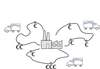
Sometimes visiting all the cities is not mandatory. In the prize-collecting traveling salesman problem, a revenue is attached to each city and the objective is to maximize the net revenue defined as the total collected revenue minus the total traveled distance (counting a cost of 1 per unit of distance).

This variant requires only a slight modification of the TSP model, as illustrated below.

// A list variable: cities[i] is the index of the ith city in the tour
cities <- list(nbCities);
revenue <- sum(cities, i => prize[i]);

distance <- count(cities) <= 1 ? 0 : sum(1..count(cities)-1, i => distanceWeight[cities[i-1]][cities[i]])
                + distanceWeight[cities[count(cities)-1]][cities[0]];

maximize revenue - distance;

You can observe that the contraint on the size of the list has been removed. Consequently the distance expression is modified to take into account the now possible case of empty or singleton lists. The revenue collected by the tour is measured with a simple sum. Note that the range on which the sum is applied can be defined as an interval (as in the distance case, to enumerate all positions in the list) or directly as a list (to enumerate values contained in the list).

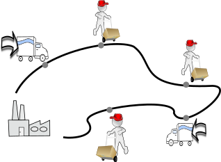
The Capacitated Vehicle Routing Problem (CVRP)¶

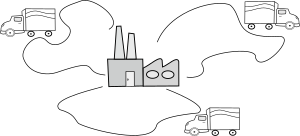
In the capacitated vehicle routing problem (CVRP), a fleet of delivery vehicles with uniform capacity must serve customers with known demand for a single commodity. The vehicles start and end their routes at a common depot and each customer must be served by exactly one vehicle.

The objective is to assign a sequence of customers to each truck of the fleet, minimizing the total distance traveled, such that all customers are served and the total demand served by each truck does not exceed its capacity.

As explained in our example tour, this problem is modeled with one list variable per truck of the fleet, and the coverage of all customers is enforced by a partition constraint:

// All customers must be visited by the trucks
constraint partition[k in 1..nbTrucks](tour[k]);

And the capacity contraint is modeled with a sum over all items assigned to a truck:

sequence <- tour[k];
c <- count(sequence);
routeQuantity <- sum(0..c-1, i => demands[sequence[i]]);
constraint routeQuantity <= truckCapacity;

Many test cases of this capacitated vehicle routing problem are available in the literature. Our CVRP benchmark page shows how quickly LocalSolver finds high-quality solutions to these problems.

The Prize-Collecting Capacitated Vehicle Routing Problem (PCCVRP)¶

In the prize-collecting variant of the capacitated vehicle routing problem, instead of serving all customers (which may be impossible due to a limited fleet for instance), the goal is to maximize the total collected revenue.

In this context, the lists will not form a partition of the set of all customers, but it is still forbidden to have more than one truck visiting the same customer. Therefore the partition contraint becomes a disjoint constraint:

// At most one visiting truck per customer
constraint disjoint[k in 1..nbTrucks](customersSequences[k]);

The remainder of the model is unchanged except for the objective function that now measures the total collected revenue, defined on each tour as sum(tour[k], i => prize[i]).

The Capacitated Vehicle Routing Problem with Time-Windows (CVRPTW)¶

Handling time-windows in routing problems means ensuring that each delivery takes place in a given time-window.

In many cases (for example in the standard CVRPTW), it can be modeled without introducing delivery times as decision variables. Indeed, a key modeling principle is to avoid introducing a decision when an expression can in fact be inferred from other expressions. It is the case for the CVRPTW, where the delivery time for a customer can be defined as the maximum of:

the earliest allowed delivery time for this customer

the departure time from the previous customer plus the travel time to the current customer

This definition is recursive and can be modeled in LocalSolver by means of a function (i, prev) => .... These functions are used to define the i-th element of an array as a function of the (i-1)-th element and the value i. See our documentation on this topic for details:

endTime[k] <- array(0..c-1, (i, prev) => max(earliestStart[sequence[i]],
                      i == 0
                          ? distanceWarehouse[sequence[0]]
                          : prev + distanceMatrix[sequence[i-1]][sequence[i]])
                  + serviceTime[sequence[i]]);

The lateness at each customer is computed as the difference between the ending time of this visit and the latest allowed end for this customer. For the arrival at the depot, we compare the arrival time to the maximum horizon defined for the problem.

Our example tour includes a detailed model for this problem with sample data and ready-to-use code in LSP, C++, Java, .NET and Python.

CVRP with preassignments¶

Sometimes some visits are preassigned to a given truck. On the contrary, we can also have some visits that cannot be assigned to some trucks (for example because of the size of the truck or because of the clearances of the driver).

Such constraints can easily be defined on list variables thanks to the contains operator:

// with mandatory and forbidden defined as maps of pairs truck/visit
for[req in mandatory] constraint contains(tour[req.truck], req.visit);
for[req in forbidden] constraint !contains(tour[req.truck], req.visit);

The Pickup and Delivery Problem (PDVRP)¶

In the pickup-and-delivery problem, the items to be delivered are not loaded into the truck at the depot before starting the tour, but they are collected along the tour. In other words, each demand is made of a pickup point (where the item will be collected) and a delivery point (where the item will be delivered).

This situation induces three constraints:

Each pickup/delivery pair must be assigned to the same tour,

Within this tour, the pickup cannot be visited after the delivery (an item that is yet to be picked up cannot be delivered),

The weight of the truck will vary along the tour (increasing upon pickups and decreasing upon deliveries) and the capacity constraint must be satisfied at any time during the tour.

Considering each list in the LocalSolver model, the first requirement for a pickup/delivery pair (a,b) means that a and b either both belong to the list or none of them belong to the list. Literally it means that contains(sequence[k], a) == contains(sequence[k], b).

As for the ordering of the pair within the list, it is related to the position of a and b within the list, which can be obtained with the indexOf operator:

for[k in 1..nbTrucks] {
      constraint contains(sequence[k], a) == contains(sequence[k], b);
      constraint indexOf(sequence[k], a) <= indexOf(sequence[k], b);
}

Note that indexOf takes the value -1 when searching for an item that is not contained in the list. Consequently writing a strict inequality on the second constraint would be an error because it would not allow both items to be outside the list.

As mentioned above, the last specificity is that the capacity constraint must now be checked after each visit. To do this, we need to define the weight after a visit as the weight before the visit plus the weight of the current item (positive if loaded, negative if delivered):

for[k in 1..nbTrucks] {
    weight[k] <- array(0..c-1, (i, prev) => prev + demands[sequence[i]]);
    constraint and(0..c-1, i => weight[k][i] <= truckCapacity);
}

CVRPTW with minimization of waiting time¶

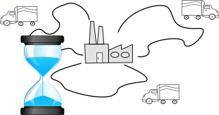
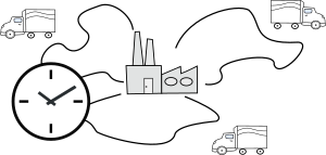
In the CVRPTW the usual objective is to minimize the total traveled time. In this context, the satisfaction of time-window constraints is optimal with an earliest scheduling approach (starting the tour at the earliest possible date).

However, this strategy can lead to unnecessary waiting time for drivers. Hence an additional requirement is sometimes to minimize the total waiting time, or (equivalently) to minimize the total duration of tours.

A simple approach can be to introduce a startTime[k] integer decision variable for each tour k. In the CVRPTW model, it will just be added to the initial travel time from the depot for each tour.

Alternatively, we show below that introducing these decisions can be avoided, thanks to a careful computation of the minimum waiting time for a tour. To achieve this, we compute the earliest scheduling of the tour as in the classical CVRPTW and we maintain alongside the maximum shifting of the starting time of the tour that is still possible without visiting a customer too late. This margin array is recursively computed based on the following definitions:

We define the arrival as the earliest arrival time on site (endTime of previous visit plus travelTime)

We define the earliness as the time from arrival to the start of the time-window (0 if arrivalTime is within the time-window)

We define the slack as the difference between endTime and the end of the time-window

Regular arrival

Early arrival

The rationale of the model is the following:

If earliness is zero then we just observe the slack on this time-window. If smaller than the current margin, then we register this slack as the maximum possible shifting of the start of the tour: margin <- min(margin, slack).

If earliness is non-zero then we try to absorb this earliness by shifting the starting time of the shift. If the current margin is larger than this earliness, then the residual margin is now min(margin-earliness, slack). Otherwise we do not have enough margin to avoid a waiting time of earliness-margin on this site. From this point, any earliness will be unavoidable waiting time.

The LSP code below implements this strategy. In this model, negative values of margin[i] code for the waiting time before visit i:

 for[k in 0..nbTrucks-1] {
      local sequence <- tour[k];
      local c <- count(sequence);

      // A truck is used if it visits at least one customer
      truckUsed[k] <- c > 0;

      endTime[k] <- array(0..c-1, (i, prev) => max(timeWindowsLB[sequence[i]],
                            i == 0
                                ? travelTimeMatrixFromDepot[k][sequence[0]]
                                : prev + travelTimeMatrix[sequence[i-1]][sequence[i]])
                        + handlingTime[sequence[i]]);

     arrivalTime[k] <- array(0..c-1, i =>
                            i == 0
                                ? endTime[k][i]-handlingTime[sequence[i]]
                                : endTime[k][i-1] + travelTimeMatrix[sequence[i-1]][sequence[i]]);

      // If margin[k][i] > 0, it represents the remaining margin after visit i
      // otherwise, -margin[k][i] is the waiting time for visit i
      margin[k] <- array(0..c-1, (i, prev) =>
                                i == 0 ?
                                    // We can always absorb the time on the first node
                                    // (because we can delay the departure to not wait).
                                    slack(k,0)
                                    :
                                    // Not the first node
                                    prev > 0
                                        // We still have some margin, we absorb earliness
                                        ? min(prev - earliness(k,i), slack(k,i))
                                        // We don't have any margin, we wait if we arrive early
                                        : -earliness(k,i));

      // Total time that driver k waits on day d during his route
      waitingTime[k] <- sum(0..c-1, i => max(-margin[k][i], 0));
}

function earliness(k, i) { return max(0,timeWindowsLB[tour[k][i]] - arrivalTime[k][i]);}
function slack(k, i) { return timeWindowsUB[tour[k][i]] - endTime[k][i];}

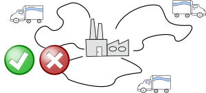
TSP with draft limits (TSPDL)¶

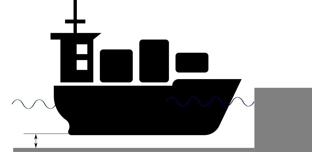
The draft of a ship is the distance between the waterline and the bottom of the ship. This draft increases with the load of the ship and each port has a draft limit, beyond which a vessel cannot enter the port. Hence in maritime transportation the ability to visit a site depends on the amount of carried cargo.

Such a limitation can occur in other contexts where the accessibility of a site depends on the weight of the vehicle. As in the pickup and delivery problem, it requires computing the weight of the vehicle along the tour:

weight <- array(0..c-1, (i, prev) => i == 0
                            ? totalWeight
                            : prev - itemWeight[sequence[i-1]]);

// Setting a contraint over all terms of an array is done with the 'and' operator:
constraint and(0..c-1, i => weight[i] <= weightLimit[sequence[i]]);

// Altenatively (for instance if finding a solution respecting all draft limits
// take more than a few seconds), you can minimize the cumulated overweight:
overweight <- sum(0..c-1, i => max(0, weight[i] - weightLimit[sequence[i]]));