Modeling and Solving Curve Fitting Problems

LocalSolver solves combinatorial but also continuous optimization problems. Here we show how Curve Fitting problems can be easily modeled and optimally solved, in seconds, using LocalSolver Optimizer. Curve Fitting consists in constructing a curve that best fits a series of data points. A pair of input and output define each data point. The curve corresponds to a mathematical function. Considering a given form for the mapping function, we want to find its optimal parameters to best map inputs into the set of outputs.

Linear fitting
For example, for this dataset, we assume the mapping function has the form f(x) = a*x + b, and we want to find the parameters a and b for which the mapping function fits best the observations, which means that the error of prediction by the mapping function is the smallest. The LocalSolver model presented here is implemented in Python. The decision variables are the parameters of the mapping function: a, b. We want these variables to be continuous and between -100 and +100.
# Decision variables: parameters of the mapping function
a = model.float(-100, 100)
b = model.float(-100, 100)
The objective is to minimize the sum of square errors: the square error is the square difference between the output predicted by the mapping function and the observed output for a given input.
# Minimize square error between prediction and output
predictions = [a * inputs[i] + b for i in range(nb_observations)]
errors = [predictions[i] - outputs[i] for i in range(nb_observations)]
square_error = model.sum(model.pow(errors[i], 2) for i in range(nb_observations))
model.minimize(square_error)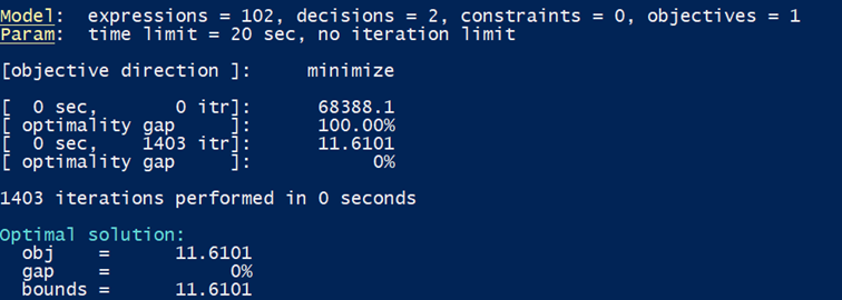
LocalSolver finds the optimal solution immediately. The figure below shows the function solution of the problem.

Polynomial fitting
We want to try with a polynomial mapping function of the form: f(x) = a*x3 + b*x2 + c*x + d. We only have to change the decision variables:
a = model.float(-100, 100)
b = model.float(-100, 100)
c = model.float(-100, 100)
d = model.float(-100, 100)
and the computation of predictions:
predictions = [a *inputs[i]**3 + b * inputs[i]**2 + c * inputs[i] + d for i in range(nb_observations)]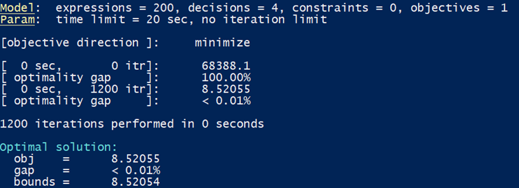
Again, LocalSolver finds the optimal solution immediately. The figure below shows the function solution of the problem. We see that it fits best the data series than the linear function. But the function cannot catch the periodic variations of the observations. Thus, we are going to try a function with a sinusoidal part.

Nonlinear fitting
We now suggest a nonlinear mapping function of the form: f(x) = a*sin(b-x) + c*x + d. We only have to change the decision variables:
a = model.float(-10, 10)
b = model.float(0, 2*math.pi)
c = model.float(-100, 100)
d = model.float(-100, 100)
and the computation of predictions:
predictions = [a * model.sin(b - inputs[i]) + c * inputs[i] + d for i in range(nb_observations)]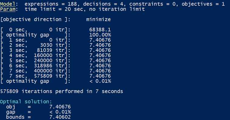
LocalSolver finds the optimal solution immediately but needs a few seconds to prove it. The figure below shows the function solution of the problem.

You can find the complete model of the Curve Fitting problem in Python, Java, C#, and C++ in our Example Tour.
We are at your disposal to accompany you in the discovery of LocalSolver. Don’t hesitate to contact us for any further information or support.