Piecewise operator
Piecewise linear functions are introduced in LocalSolver with the piecewise
operator. A piecewise linear function is a function composed of straight-line
sections. The extremities of each straight-line are called breaking points.
We define a piecewise function by giving all its breaking points in left to
right order.
The piecewise operator takes exactly 3 arguments:
A non-decreasing array of ‘’n’’ constant numbers, with ‘’n’’ >= 2.
An array of ‘’n’’ constant numbers.
An integer or double expression.
The solution will be infeasible if the value of the third operand is strictly smaller that the first element of the first array, or strictly larger than the last element of the first array. This operator returns a floating number.
The expression piecewise(x,y,z) returns the image of z by the function
defined by geometric points (x[0], y[0]), (x[1], y[1]), ..... (x[n-1], y[n-1]).
For instance piecewise({0, 50, 100}, {0, 10, 100}, 75) returns 55.
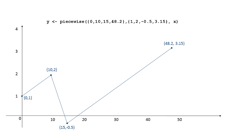
The figure below illustrates the curve defined by
y <- piecewise({0,10,15,48.2},{1,2,-0.5,3.15}, x).
Note that this expression returns an undefined value when x < 0 or x > 48.2.
In this case, if this undefined value is used (directly or indirectly) in an
objective or a constraint, the solution will be considered invalid.
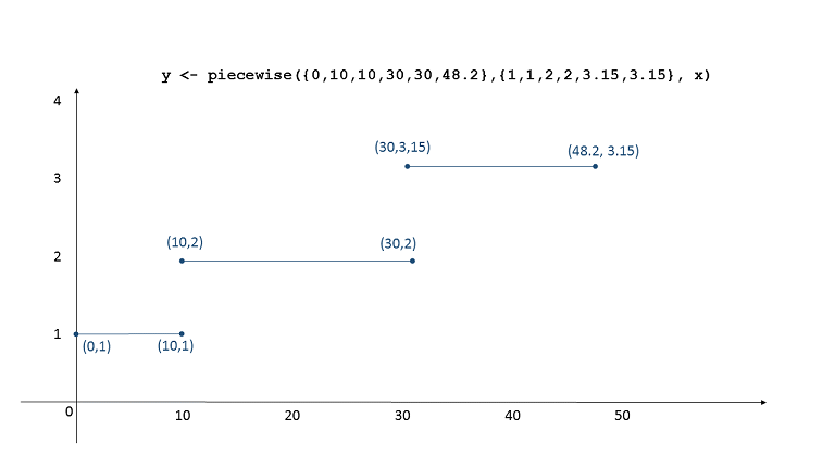
Discontinuities are allowed in the definition of the function, that is to say that two geometric points can share the same x-coordinate. By convention the value taken by the function at such a discontinuous point is the one associated to the last occurrence of this x-coordinate in array.
For instance piecewise({0, 50, 50, 100}, {0, 0.1, 0.9, 1}, 50) returns 0.9.
The figure below illustrates the curve defined by
y <- piecewise({0 ,10 ,10 ,30 ,30 , 48.2}, {1 , 1, 2, 2, 3.15, 3.15}, x).
This stepwise shape is often useful but any other discontinuous linear
functions are allowed.